DeepSeek’s Visual Primitives and the Missing Layer in Multimodal Reasoning

Note: This article discusses Thinking with Visual Primitives, a DeepSeek paper that is no longer available at its original location. The architecture, training details, and benchmark results reported here come from the version we reviewed. We have not independently reproduced those results.

A multimodal model can recognize every person in a crowded photograph and still count the group incorrectly.

The problem may appear perceptual. Perhaps the people are too small, the image is too compressed, or the visual encoder missed someone. Those failures are real. They belong to what Thinking with Visual Primitives calls the Perception Gap.

A separate failure occurs after perception. The model sees a person, describes that person in language, moves to another part of the image, and later loses track of who has already been counted. The paper calls this loss of stable object identity across a reasoning trace the Reference Gap.

Its proposed solution is surprisingly direct. Let the model place a bounding box around an object while reasoning about it. Let it emit points while following a path. Interleave those coordinates with language so that “this person,” “that bear,” and “the current branch of the maze” have exact spatial handles.

A box becomes working memory for an object. A point sequence becomes working memory for a path.

That idea matters more than any single score in the paper. Multimodal reasoning needs a representation for spatial state. Language can describe that state, but descriptions become ambiguous in crowded scenes, overlapping layouts, long trajectories, and multi-step deductions. Visual primitives give the reasoning process something closer to a coordinate system.

Seeing and referring are different operations

The paper illustrates fine-grained counting with a wildlife image containing bears on rocky terrain and a bear climbing a tree. It asks the model to count only the bears standing on the terrain.

This requires a procedure:

• Find every bear.
• Preserve the identity of each candidate.
• Determine whether the bear is standing on earth or rocks rather than climbing the tree.
• Exclude the climbing bear.
• Count the remaining set.

A global image description is a poor data structure for this procedure. “There are several bears, including one near a tree” does not tell the next reasoning step which bear has already been evaluated.

A set of grounded objects does. After grounding, the candidate set is $\mathcal B_{\text{bear}}=\{b_1,b_2,\ldots,b_n\}$, where each box has coordinates $b_i=\left(x_i^{(1)},y_i^{(1)},x_i^{(2)},y_i^{(2)}\right)$ for its two corners.

The corners $(x_i^{(1)},y_i^{(1)})$ and $(x_i^{(2)},y_i^{(2)})$ identify the top-left and bottom-right of one candidate. The conditional count becomes

$$\hat y = \sum_{b_i\in\mathcal B_{\text{bear}}} \mathbf 1\!\left[g(I,b_i)=1\right],$$

where $I$ is the image and $g(I,b_i)$ tests whether the bear inside box $b_i$ is supported by the rocky terrain rather than clinging to the tree.

This formalization separates three sources of error:

• Grounding error: $\mathcal B_{\text{bear}}$ contains a missing, duplicated, or incorrect box.
• Predicate error: $g(I,b_i)$ misclassifies a grounded bear.
• Aggregation error: the final sum is inconsistent with the filtered set.

The decomposition is useful even when the final answer is wrong. It tells us whether the model lost the object, misunderstood the relation, or failed to count its own candidates.

This is the practical meaning of the Reference Gap. Perception asks whether the evidence entered the model. Reference asks whether later computation can keep addressing the same evidence.

The primitive language

The paper uses bounding boxes for identifiable objects and points for abstract locations and trajectories.

A box response follows this grammar:

<|ref|>TARGET<|/ref|>
<|box|>[[x1,y1,x2,y2],[x3,y3,x4,y4],...]<|/box|>

A point response follows:

<|point|>[[x1,y1],[x2,y2],...]<|/point|>

Multiple boxes are ordered from left to right. Point sequences omit the object name, allowing the same format to represent a center point, a maze step, or a trajectory through a tangled curve.

All coordinates are quantized to integers from 0 to 999. For an image with width $W$ and height $H$, a natural implementation is

$$\begin{aligned} q_x&=\operatorname{round}\!\left(999\frac{x}{W-1}\right),\\ q_y&=\operatorname{round}\!\left(999\frac{y}{H-1}\right). \end{aligned}$$

The approximate inverse is

$$\begin{aligned} \hat x&=\frac{q_x}{999}(W-1),\\ \hat y&=\frac{q_y}{999}(H-1). \end{aligned}$$

Rounding introduces a bounded error. If $q_x$ is the nearest integer, then

$$\begin{aligned} |\hat x-x|&\leq\frac{W-1}{2\cdot999},\\ |\hat y-y|&\leq\frac{H-1}{2\cdot999}. \end{aligned}$$

For a 1,000-pixel-wide image, the horizontal quantization error is at most about half a pixel. For a 4K image, it can approach two pixels. Resizing and padding can introduce additional error, so coordinate normalization does not make the entire vision pipeline resolution invariant. It only gives the emitted primitives a fixed vocabulary.

from dataclasses import dataclass

GRID_MAX = 999


def quantize(value: float, extent: int) -> int:
    if extent < 2:
        raise ValueError("extent must be at least 2")
    value = min(max(value, 0.0), extent - 1)
    return round(GRID_MAX * value / (extent - 1))


def dequantize(value: int, extent: int) -> float:
    if not 0 <= value <= GRID_MAX:
        raise ValueError("coordinate must be in [0, 999]")
    return value * (extent - 1) / GRID_MAX


@dataclass(frozen=True)
class Box:
    x1: int
    y1: int
    x2: int
    y2: int

    def validate(self) -> None:
        values = (self.x1, self.y1, self.x2, self.y2)
        if any(v < 0 or v > GRID_MAX for v in values):
            raise ValueError("box coordinates must be in [0, 999]")
        if self.x1 > self.x2 or self.y1 > self.y2:
            raise ValueError("box corners are reversed")

The syntax is simple enough to parse and render. That is an important property. A reasoning trace becomes a machine-checkable interface rather than free-form prose alone.

Counting becomes ground, filter, tally

The paper divides counting into coarse and fine-grained tasks.

Coarse counting asks for a general category, such as the number of people. Its procedure is batch-oriented: ground every candidate at once, then sum the boxes. Fine-grained counting adds a predicate, such as “white dogs” or, in the paper’s wildlife example, “bears standing on rocky terrain rather than climbing a tree.” Its procedure grounds a broader candidate set, evaluates the condition for each candidate, removes hard negatives, and tallies the survivors.

We can write the process as set construction:

$$\begin{aligned} \mathcal C_q(I)&=\{b_i:\operatorname{category}(I,b_i)=q\},\\ \mathcal F_{q,r}(I)&=\{b_i\in\mathcal C_q(I):r(I,b_i)=1\},\\ \hat y&=|\mathcal F_{q,r}(I)|. \end{aligned}$$

Here $q$ is the requested category and $r$ is the requested relation or attribute. For ordinary counting, $r\equiv1$, so every grounded candidate survives.

This representation does not solve recognition by itself. A perfect set of dog boxes cannot determine which dogs are Chihuahuas unless the visual encoder and predicate classifier preserve the necessary detail. Boxes reduce referential ambiguity while semantic classification still depends on visual detail.

That limitation is central to the paper’s own discussion. It reports that input resolution still constrains fine-grained performance and can produce imprecise primitives. Reference mechanisms therefore complement perceptual improvements and continue to depend on them.

A smooth reward for counting

Exact match gives the same reward to an answer off by one and an answer off by fifty: zero. The paper instead uses an exponential function of relative error:

$$R_{\text{count}}(\hat y,y) = \alpha \exp\!\left( -\beta\frac{|\hat y-y|}{|y|+1} \right),$$

Here $\alpha=0.7$ and $\beta=3$. The maximum is $\alpha$, reached when $\hat y=y$. The other reward components can still contribute to the total training signal.

Suppose the correct count is two and the model predicts three:

$$\begin{aligned} R_{\text{count}}(3,2) &=0.7\exp\!\left(-3\cdot\frac{1}{3}\right)\\ &=0.7e^{-1}\approx0.258. \end{aligned}$$

Now suppose the correct count is 100 and the model predicts 101:

$$\begin{aligned} R_{\text{count}}(101,100) &=0.7\exp\!\left(-3\cdot\frac{1}{101}\right)\\ &\approx0.679. \end{aligned}$$

This scale-sensitive behavior is intentional and generally useful when training across a wide range of counts. For a true count of two, the normalized error is $1/3$, so the reward is about 37% of its maximum value. For a true count of 100, the normalized error is only $1/101$, so the reward remains about 97% of its maximum. The second prediction is still incorrect, but it is much closer relative to the size of the target count.

from math import exp


def counting_reward(predicted: int, truth: int,
                    alpha: float = 0.7,
                    beta: float = 3.0) -> float:
    relative_error = abs(predicted - truth) / (abs(truth) + 1)
    return alpha * exp(-beta * relative_error)

Points turn a visual maze into a state trace

Bounding boxes fit object-centric reasoning, while a maze is better described through connectivity, visited locations, branches, and reachability.

Represent the maze as a graph $G=(V,E)$, where every traversable region is a vertex and every legal move is an edge. A model-generated exploration is the sequence $\tau=(v_0,v_1,\ldots,v_T)$.

For each transition, $\ell_t=\mathbf 1[(v_t,v_{t+1})\in E]$ records whether the move is legal. The first wall violation is $t^\star=\min\{t:\ell_t=0\}$. If no violation occurs, set $t^\star=T$. The causally valid prefix is $\tau_{\text{valid}}=(v_0,v_1,\ldots,v_{t^\star})$.

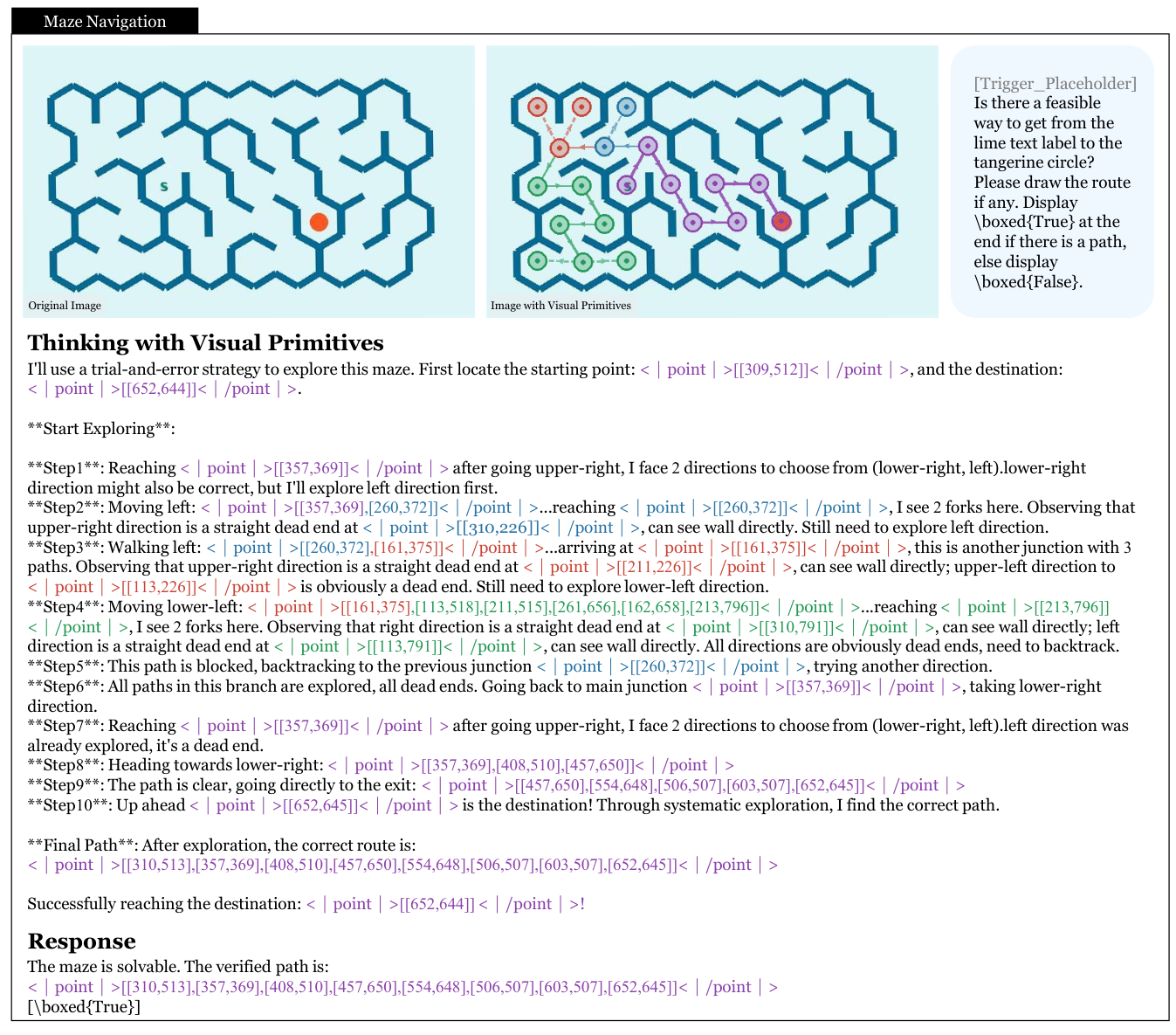
This truncation rule is one of the paper’s better reward-design choices. Once a trace crosses a wall, later locations cannot be credited as valid exploration. The model reached them through an impossible transition.

The paper describes five maze-reward components but does not print their complete weighted equation. The following is a faithful mathematical reconstruction of that prose. The notation and composition are ours; the underlying components come from the paper.

For a solvable maze, let $g$ be the goal, $L^\star$ the length of a ground-truth path, and $S_{\text{valid}}$ the set of vertices in the valid prefix. If $d_{\min}=\min_{v\in S_{\text{valid}}}d_G(v,g)$ is the closest legal approach to the goal, define progress as

$$R_{\text{progress}} = \operatorname{clip}\!\left(1-\frac{d_{\min}}{L^\star},0,1\right),$$

where $d_G$ is shortest-path distance in the maze graph.

For an unsolvable maze, let $\mathcal R(v_0)$ be every vertex legally reachable from the start. Exploration completeness is

$$R_{\text{complete}} = \frac{|S_{\text{valid}}\cap\mathcal R(v_0)|} {|\mathcal R(v_0)|}.$$

If $N_{\text{wall}}$ is the number of illegal transitions in the full generated trace and $N_{\text{legal}}$ is the number of legal transitions available in the maze, the described wall score can be written as

$$R_{\text{wall}} = \operatorname{clip}\!\left( 1- \frac{N_{\text{wall}}}{N_{\text{legal}}}, 0, 1 \right).$$

The claimed final path receives

$$\begin{aligned} R_{\text{path-valid}}=\mathbf 1\!\Bigl[& \hat v_0=v_0,\ \hat v_K=g,\\ &\forall k:(\hat v_k,\hat v_{k+1})\in E \Bigr]. \end{aligned}$$

Answer correctness is $R_{\text{answer}}=\mathbf 1[\hat s=s]$, where $s$ is the true solvability label.

A generic weighted composition is

$$\small \begin{aligned} R_{\text{maze}}={}& \lambda_pR_{\text{progress}} +\lambda_cR_{\text{complete}} +\lambda_wR_{\text{wall}}\\ &+\lambda_vR_{\text{path-valid}} +\lambda_aR_{\text{answer}}. \end{aligned}$$

The paper does not disclose these $\lambda$ values. It also sets inapplicable components to one. Progress applies to solvable mazes, while completeness applies to unsolvable ones.

The conceptual advantage is dense feedback. A binary final answer only says whether the maze was classified correctly. This reward can distinguish legal exploration, useful progress, comprehensive failure analysis, wall violations, and a valid final route.

Path tracing is geometry, not description

A tangled-line puzzle makes the Reference Gap easy to see. Try describing a target curve with prose:

Move upward, bend right, pass beneath the crossing, turn left, and continue toward the purple icon.

Every phrase depends on a current position that language does not preserve exactly. A point sequence $\hat P=(\hat p_1,\hat p_2,\ldots,\hat p_M)$, with each $\hat p_i\in[0,999]^2$, carries that state directly.

The paper samples fewer waypoints on straight sections and denser waypoints near sharp curves and intersections. This resembles adaptive numerical integration: allocate more samples where local geometry changes quickly.

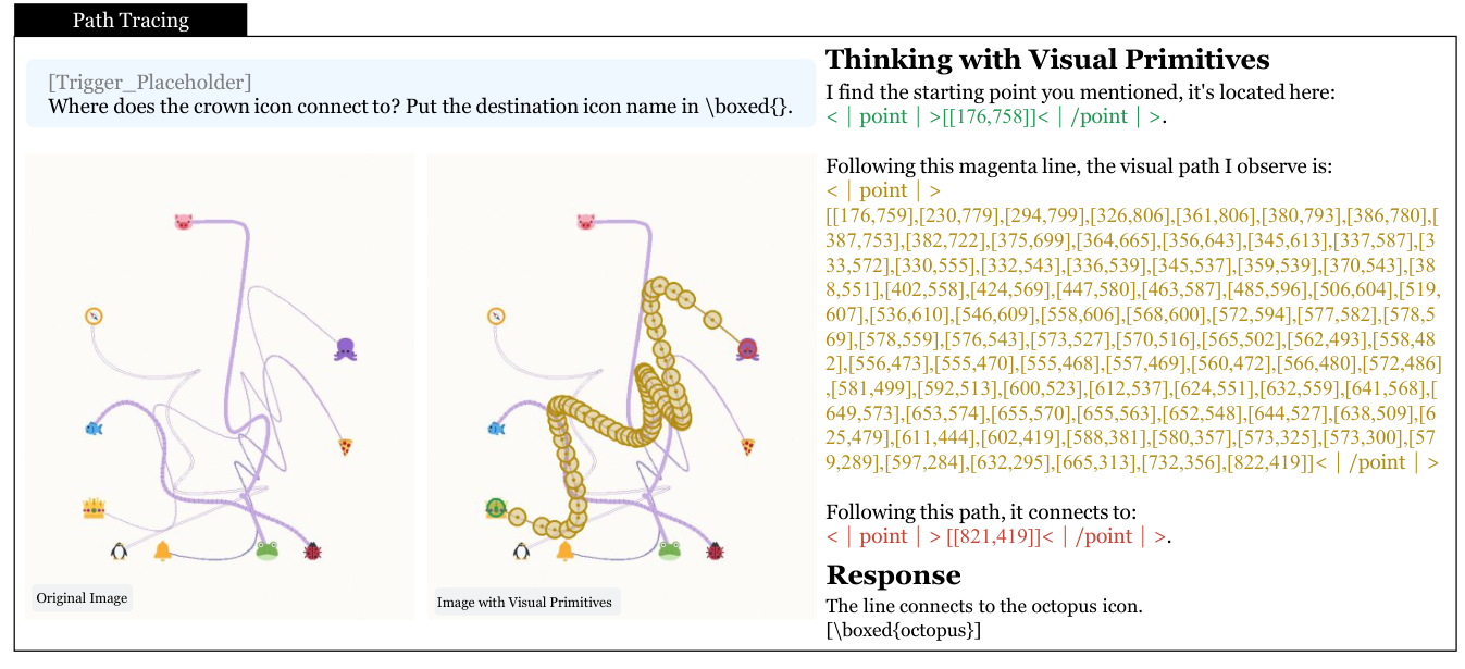
Scoring such a trace requires more than checking its endpoint. A model could guess the correct destination without following the line. It could also emit a few safe points near the start and stop.

Distance from a point to a segment

For point $p$ and line segment with endpoints $a$ and $b$, project $p$ onto the infinite line, clamp the coefficient to the segment, and then measure the distance to the resulting closest point:

$$\begin{aligned} u&=\frac{(p-a)^\top(b-a)}{\|b-a\|_2^2},\\ u^\star&=\operatorname{clip}(u,0,1),\\ \Pi_{[a,b]}(p)&=a+u^\star(b-a),\\ d(p,[a,b])&=\left\|p-\Pi_{[a,b]}(p)\right\|_2. \end{aligned}$$

For a polyline $P=(p_1,\ldots,p_N)$, let $\operatorname{seg}(P)=\{[p_j,p_{j+1}]:1\le j<N\}$ denote its set of line segments.

Why the distance must run in both directions

Predicted-to-ground-truth error measures whether generated points stay near the true curve:

$$D_{\rightarrow}(\hat P,P) = \frac{1}{M} \sum_{i=1}^{M} \min_{s\in\operatorname{seg}(P)} d(\hat p_i,s).$$

Ground-truth-to-predicted error measures whether the generated trace covers the whole curve:

$$D_{\leftarrow}(P,\hat P) = \frac{1}{N} \sum_{j=1}^{N} \min_{\hat s\in\operatorname{seg}(\hat P)} d(p_j,\hat s).$$

The paper describes a bidirectional distance without printing its complete equation. A direct reconstruction is

$$\begin{aligned} D_{\text{bi}}(\hat P,P)=\frac{1}{2}\Bigl(& D_{\rightarrow}(\hat P,P)\\ &+D_{\leftarrow}(P,\hat P) \Bigr). \end{aligned}$$

A short safe trace can score well in the forward direction because every predicted point lies near the correct curve, while its reverse error remains large because most of the true curve has no nearby prediction. A long detour can improve reverse coverage by passing near much of the correct curve, but its off-curve points increase the forward error. Scoring in both directions prevents either shortcut from receiving a high reward.

import numpy as np


def point_segment_distance(p, a, b) -> float:
    p = np.asarray(p, dtype=float)
    a = np.asarray(a, dtype=float)
    b = np.asarray(b, dtype=float)
    ab = b - a
    denom = float(ab @ ab)
    if denom == 0.0:
        return float(np.linalg.norm(p - a))
    u = np.clip(((p - a) @ ab) / denom, 0.0, 1.0)
    projection = a + u * ab
    return float(np.linalg.norm(p - projection))


def directed_polyline_distance(points, target_polyline) -> float:
    segments = list(zip(target_polyline[:-1], target_polyline[1:]))
    distances = [
        min(point_segment_distance(p, a, b) for a, b in segments)
        for p in points
    ]
    return float(np.mean(distances))


def bidirectional_distance(predicted, truth) -> float:
    forward = directed_polyline_distance(predicted, truth)
    reverse = directed_polyline_distance(truth, predicted)
    return 0.5 * (forward + reverse)

The paper adds endpoint accuracy, a continuity penalty, and endpoint-label correctness. Let $c_s$ and $c_e$ be the ground-truth centers of the start and end boxes. We use $\hat e$ for the endpoint coordinate that the model declares separately from the last waypoint $\hat p_M$ in its generated trace. If $\phi(d;\delta)$ is a distance-decay function that reaches zero at tolerance $\delta$, then an explanatory reconstruction is

$$\begin{aligned} R_{\text{start}}&=\phi(\|\hat p_1-c_s\|_2;\delta_s),\\ R_{\text{end}}&=\phi(\|\hat e-c_e\|_2;\delta_e). \end{aligned}$$

A jump is penalized when $P_{\text{jump}}=\mathbf 1[\|\hat p_M-\hat e\|_2>\delta_c]$ evaluates to one. If $\hat \ell$ is the endpoint label in the model's final answer and $\ell^\star$ is the ground-truth endpoint label, then $R_{\text{label}}=\mathbf 1[\hat \ell=\ell^\star]$.

A generic reconstruction of the final path reward is

$$\begin{aligned} R_{\text{trace}}={}& \lambda_\tau\psi(D_{\text{bi}}) +\lambda_sR_{\text{start}} +\lambda_eR_{\text{end}}\\ &+\lambda_aR_{\text{label}} -\lambda_cP_{\text{jump}}. \end{aligned}$$

The paper does not specify $\phi$, $\psi$, the tolerances, or the component weights. Those details matter for reproduction. The published description still reveals the intended geometry: stay on the curve, cover the curve, reach the correct endpoint, and do not jump there from an incomplete trace.

Model architecture and visual token compression

The paper explicitly describes the model as using “a standard architecture similar to LLaVA.” DeepSeek-ViT encodes the image. The resulting visual tokens are concatenated with text tokens and passed into DeepSeek-V4-Flash, a mixture-of-experts language model described as having 284 billion total parameters and 13 billion active parameters during inference.

The visual pipeline is aggressively compressed. For a 756 by 756 image with 14 by 14 patches, the patch count is $N_{\text{patch}}=(756/14)^2=54^2=2916$. A 3 by 3 spatial merge combines nine adjacent patches, giving $N_{\text{visual}}=2916/9=324$. Compressed Sparse Attention then reduces the visual KV entries by another factor of four, so $N_{\text{KV}}=324/4=81$.

Relative to storing one KV entry for every patch token, the cache-entry reduction is $2916/81=36$. The paper also reports $(756\cdot756)/81=7056$ raw pixels per final visual KV entry. That ratio is useful for intuition, but pixels and KV entries are different representational units. It should not be interpreted as a direct information-compression measurement.

This efficiency creates an unresolved question. At what point does better reference stop compensating for reduced perception? The paper does not provide the visual-token-budget ablation needed to answer it.

Data curation at scale

The paper reports 97,984 box-grounding data sources collected from the web. Semantic review retains 43,141. Geometric and completeness review retains 31,701. Category-balanced sampling with global deduplication produces over 40 million samples.

The post-training cold-start data contains approximately:

Most of this specialized corpus targets topology. That distribution matters when interpreting the reported maze and path results.

The full training pipeline has five stages

The sequence moves from shared pretraining through specialization and back to one unified model:

1. Pretraining teaches the primitive grammar.
2. Specialized SFT produces a grounding model $F_{\mathrm{TwG}}$ and pointing model $F_{\mathrm{TwP}}$.
3. Specialized RL optimizes each model with GRPO.
4. Unified rejection fine-tuning merges expert-generated data.
5. On-policy distillation transfers both expert distributions into one student.

The paper says that separating boxes and points during early post-training prevents mode conflict when specialized data is limited. The two outputs differ structurally: a box is a fixed four-coordinate object reference, while a point trace is a variable-length geometric sequence with different output statistics and verification rules.

For a supervised response $y=(y_1,\ldots,y_T)$ containing language and primitive tokens, the standard autoregressive SFT objective is

$$\mathcal L_{\mathrm{SFT}}(\theta) = -\sum_{t=1}^{T} \log\pi_\theta \left(y_t\mid I,q,y_{<t}\right),$$

where $I$ is the image and $q$ is the instruction. The paper does not print the SFT loss, so this is the conventional objective implied by the described training stage.

During specialized RL, intermediate boxes and points are not directly supervised. The data only needs images, questions, and final answers. Format, quality, and task-specific reward models evaluate the generated traces. This makes RL data easier to scale, while placing considerable pressure on reward design.

For a group of $G$ responses with rewards $r_1,\ldots,r_G$, GRPO begins with a relative advantage such as

$$A_i = \frac{r_i-\bar r}{s_r+\varepsilon}, \qquad \bar r=\frac{1}{G}\sum_{j=1}^{G}r_j,$$

where $s_r$ is the within-group reward standard deviation. Define the likelihood ratio as

$$\rho_{i,t}(\theta) = \frac{\pi_\theta(y_{i,t}\mid h_{i,t})} {\pi_{\theta_{\mathrm{old}}}(y_{i,t}\mid h_{i,t})}.$$

A conventional clipped group-relative objective can then be written as

$$\small \begin{aligned} \mathcal L_{\mathrm{GRPO}}(\theta)={}& -\frac{1}{G}\sum_{i=1}^{G}\frac{1}{T_i}\sum_{t=1}^{T_i}\\ &\min\!\Bigl( \rho_{i,t}A_i,\\ &\qquad\operatorname{clip}(\rho_{i,t},1-\epsilon,1+\epsilon)A_i \Bigr)\\ &+\beta_{\mathrm{KL}}D_{\mathrm{KL}}(\pi_\theta\|\pi_{\mathrm{ref}}). \end{aligned}$$

The paper says it follows the DeepSeek-V4-Flash GRPO configuration and hyperparameters, but it does not print the objective. The equations above explain the optimization family rather than document an exact implementation.

The format reward checks syntax and duplicate boxes. The quality reward uses a generative model to evaluate redundancy, consistency, contradictions, meaningful references, and reward hacking. The accuracy reward changes by task.

Before GRPO, each SFT specialist generates $N$ rollouts per sample. If $k$ is the number of correct rollouts, the paper defines difficulty as

$$\operatorname{level}(k)= \begin{cases} \text{easy}, & k=N,\\ \text{normal}, & 1\le k<N,\\ \text{hard}, & k=0. \end{cases}$$

The RL stage selects normal examples. These groups contain both successful and failed responses, giving the relative optimizer a useful learning signal.

After specialized RL, the expert models $E_{\mathrm{TwG}}$ and $E_{\mathrm{TwP}}$ generate rejection-fine-tuning data. The unified RFT stage keeps all normal examples and a random 5% of easy examples.

On-policy distillation consolidates both primitive modes

The unified model still trails its specialists. The final stage uses on-policy distillation. The paper gives the objective

$$\mathcal L_{\mathrm{OPD}}(\theta) = \sum_{i=1}^{N}w_iD_{\mathrm{KL}}\!\left(\pi_\theta\parallel\pi_{E_i}\right),$$

where $\pi_\theta$ is the unified student, $\pi_{E_i}$ is expert $i$, and $w_i$ controls that expert’s contribution. The implementation uses two teachers: the grounding expert and the pointing expert.

At token history $h_t$, let $r_{i,t}(v)$ be the log-probability ratio between the student and expert $i$. The full-vocabulary reverse KL is then

$$\begin{aligned} r_{i,t}(v)&=\log\frac{\pi_\theta(v\mid h_t)}{\pi_{E_i}(v\mid h_t)},\\ D_{i,t}&=\sum_{v\in\mathcal V}\pi_\theta(v\mid h_t)r_{i,t}(v). \end{aligned}$$

Here $D_{i,t}$ is the reverse KL between the student and expert $i$ at history $h_t$. Because the student generates the trajectories on-policy, a fuller explanatory objective is

$$\mathcal L_{\mathrm{on}}(\theta) = \mathbb E_{\tau\sim\pi_\theta}\!\left[\sum_{t,i}w_iD_{i,t}\right],$$

where the sum covers every generated step $1\le t\le|\tau|$ and every expert $1\le i\le N$.

This expanded expectation is our interpretation of the paper’s stated on-policy, full-vocabulary distillation procedure. The simpler distillation objective above is the one given in the paper.

The direction of the KL matters. Reverse KL weights tokens according to the student distribution. It strongly penalizes probability mass placed where an expert assigns very little probability. In practice, full-vocabulary logits give the student a dense target at every generated step, including ordinary language and primitive tokens.

What the reported results establish

For the counting benchmarks, the input is an image and a counting question, and the output is a number. These benchmarks use exact match (EM), which requires the predicted count to equal the ground-truth count. The spatial-reasoning, VQA, and topological benchmarks use accuracy, calculated as the number of correctly answered questions divided by the total number of questions. The paper reports these results for its unified model:

The paper also reports results on its in-house evaluations:

Pixmo-Count is the strongest clean public result in this subset. The largest apparent margins occur on the paper’s own maze and path-tracing evaluations. Those benchmarks contain 2,000 examples each and are generated using task methodologies closely related to the training data. They are useful targeted tests, but they cannot establish broad topological generalization on their own.

The paper also compares API models with identical prompts and upscales low-resolution benchmark images to at least 640,000 pixels. Models with configurable reasoning budgets are evaluated with a low budget. That is a reproducible choice only if the exact APIs, versions, prompts, and settings remain available. It may also affect relative performance.

The evidence supports a narrower conclusion: this full training recipe performs strongly on tasks designed around persistent spatial reference. It does not isolate the contribution of visual primitives.

A convincing causal study would hold model, data, and optimization constant while varying:

Additional ablations should vary the visual-token budget, compare boxes with points on the same tasks, and test the unified model against each specialist. The paper does not report the complete matrix.

Inspectable traces are not automatically faithful traces

A visual primitive is an explicit claim. The model says this box contains the object or this sequence follows the curve. Humans and software can inspect that claim.

Inspection improves debugging. It does not prove that the trace caused the answer.

Three outcomes remain possible:

• The primitive is correct and the final answer is wrong.
• The primitive is wrong and the final answer is correct.
• Both look plausible while the model arrived at them after deciding the answer.

The distinction is important:

$$\begin{gathered} \text{inspectability}\neq\text{faithfulness},\\ \text{faithfulness}\neq\text{correctness}. \end{gathered}$$

Rule-based verification can test geometric correctness. It can detect reversed boxes, duplicate regions, wall crossings, endpoint jumps, and incomplete coverage. Establishing causal faithfulness requires interventions: alter or remove the primitive and test whether the downstream answer changes in the predicted way.

The paper does not provide that evidence. Its traces are better described as inspectable spatial reasoning outputs.

Where visual primitives could matter next

The idea extends naturally beyond still images.

In video, a box can become a time-indexed track $\tau_i=\{(t_k,b_{i,k})\}_{k=1}^{T}$.

A point trace can become motion, gaze, contact, or camera trajectory. Persistent references could help an agent follow the same entity through occlusion, connect an action to its later consequence, and retrieve the exact moment when a relation changed.

Diagrams and interfaces offer another direct application. Arrows, wires, menu targets, and draggable controls already have geometric structure. A model that can preserve spatial handles through reasoning may be easier to validate than one that describes every action in prose.

These are extensions of the paper’s idea, not demonstrated results from the paper. They follow the same requirement: the system needs a stable way to address visual evidence across time and computation.

Visual state should survive the reasoning process

Visual primitives give a model explicit handles for state it would otherwise have to describe repeatedly in language. Boxes preserve object identity, while point sequences preserve location and continuity. Because these handles are structured, later reasoning steps can reuse them and external tools can check them.

The paper does not establish that these handles faithfully expose the model’s internal reasoning, and broad generalization remains an open question. Its concrete contribution is to represent selected visual references as state that can be carried through computation.

These primitives capture only selected parts of a frame. A more general system could encode objects, regions, relations, and uncertainty as a compact, updatable representation of the frame’s task-relevant state. The system could update that representation across time.

Boxes and points are a useful starting point for the broader research problem: finding compact visual state that preserves whatever later reasoning may need, including details whose relevance becomes clear only after reasoning begins.

Resources

• Thinking with Visual Primitives, DeepSeek. The paper's original page is no longer available.
• Video walkthrough of Thinking with Visual Primitives.
• Molmo and PixMo: Open Weights and Open Data for State-of-the-Art Vision-Language Models.
• LLaVA: Large Language and Vision Assistant.
• GQA: A New Dataset for Real-World Visual Reasoning and Compositional Question Answering.
• DeepSeekMath, which introduced Group Relative Policy Optimization.

S Nagaonkar, "DeepSeek’s Visual Primitives and the Missing Layer in Multimodal Reasoning",
VideoDB Labs, July 2026.

@article{nagaonkar2026deepseekSVisual,
  author = {S Nagaonkar},
  title = {DeepSeek’s Visual Primitives and the Missing Layer in Multimodal Reasoning},
  journal = {VideoDB Labs},
  year = {2026},
  note = {https://labs.videodb.io/research/deepseek-visual-primitives-reference-gap},
}